
")
6.18. Menu: Windows
6.18. Menu: Windows
6.18.1. Options
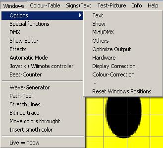
This menu and its sub-menus provide direct access to the settings in “Options” (described in chapter 6.2.5, also compare to 6.11.5 and the initial settings in chapter 2.8). It is also possible to reset the window positions through one of the sub-menus.
6.18.2. Special Functions
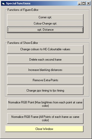
This menu item offers access to special additional features of Laserworld Showeditor. Some of these special features can be very helpful especially for the conversion of ILDA. A click on the menu item opens a dialog (Fig.62) to access the features.
The most important tools are:
● “opt. Distance” can be used for optimizing a figure. The optimization works in combination with the “Path-Tool” (See chapter 6.18.9). First apply the “opt. Distance”, then the “Path Tool” . ”Opt. Distance” splits the distances of a line into shorter pieces to sizes that match the setting in Options->Optimize Output->Max. Distance Laser ON
● “Change colors to Colortable values”: If an ILDA file with custom color palette is imported, e.g. from Pangolin, this button allows for changing the color palette to the standard Laserworld Showeditor one. After the conversion the ILDA file/frame is fully compatible for further use in Laserworld Showeditor, including saving it as *.heb file.
● “Normalize RGB Point/Frame”: This feature enhances the color values of points to achieve maximum brightness. The color values are thus adapted to the closest color with at least one laser source on full power.
Two optimization options are possible: “enhance brightest point of frame to maximum” or “enhance each point to maximal brightness”. Try the two versions on the very frame to see the results.
6.18.3. DMX
This menu item provides the same features as the “DMX” button: It opens the DMX-Window (See chapter 6.11.4).
6.18.4. Timeline
This menu item provides the same features as the “Timeline” button: It opens the Timeline window (See chapter 6.11.2).
6.18.5. Effects
This menu item provides the same features as the “Effects” button: It opens the Effects Window (See chapter 6.11.3 and 6.2.4).
6.18.6. Automatic / Sound Mode
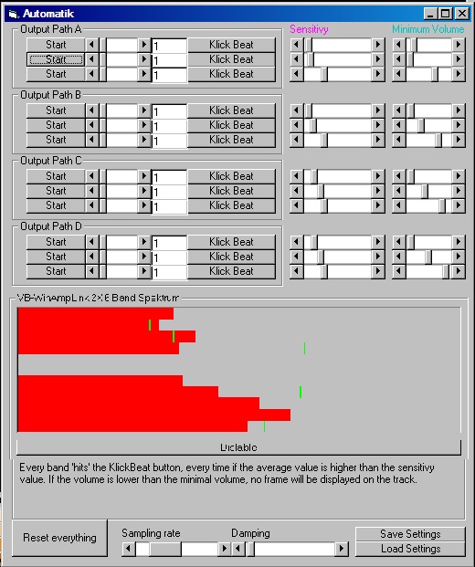
This menu item opens the window of the Automatic-Laser-Player (Fig. 68).
It offers two modes of operation:
1) Automatic Mode:
Automatic mode operation can output to paths A-D, each with 3 tracks. With rhythmically clicking on “Klick Beat”, the speed of the very output track can be specified. A generator then calls a random figure from the active Figure Table on every beat. With “Start” the output on the very track is activated.
2) Sound Mode:
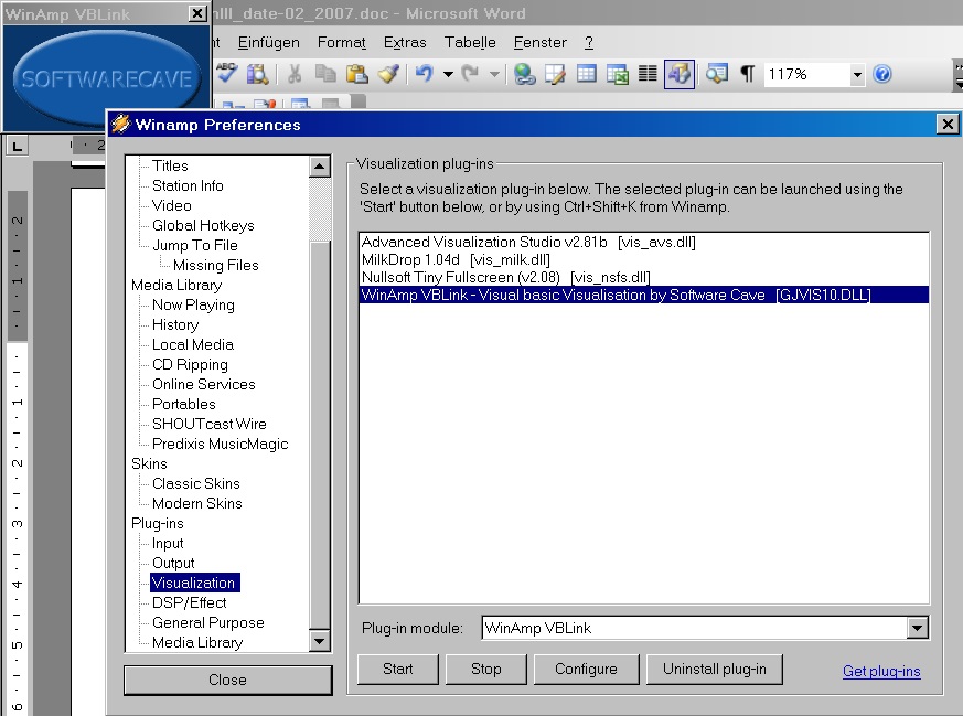
Laserworld Showeditor allows for sound active laser control in combination with WinAmp VB Link. If the music tracks are played through WinAmp, Showeditor can automatically analyse the music signal frequency and then adapt the speed of the laser figures to the beat.
To get this feature going, a WinAmp-plugin called “WinAmp VB Link” is required. It is not included with Laserworld Showeditor, but must be installed separately. It can either be downloaded form the download section on the website (http://www.showeditor.com/en/downloads) or the version included with the installation package of Laserworld Showeditor can be used.
Search for the file “vblink10.zip” within the program folder of this software. The file “readme.txt” describes the installation of the plugin. On http://www.showeditor.com there are tutorials on how to use this plugin, also on different operating systems. In some rare cases it may be necessary to use some special tricks to get the drivers working. This is explained in the tutorials.
A “Softwarecave” logo in the upper left corner shows that the plugin is active. Click “enable” in the automatic mode window, so the plugin can start to analyse the frequencies. It is necessary to start the tracks by clicking on the “Start” button of the very track. If music is playing in WinAmp, the incoming frequency tracks should be visible in the VB-WinAmp Link area. (See Fig. 69).
The assignment of the tracks to the frequencies is split by frequency range, so track A is assigned to the lower frequencies, B to the middle frequencies and D to the high ones. Six of the tracks are triggered by the left sound signal, the others are triggered by the right sound one.
Many different features and settings are possible, but the description here is kept on a basic level. It is recommended to try and find out.
The buttons “Save” and “Load” allow for saving or loading of the specific settings. “Reset everything” does a full reset of the settings, be careful. The scrollbar “Sampling Rate” sets the interval for updating the intensity value through the frequency analyser. It is recommended to increase the sampling rate value on fast computers.
LineIn Sound Mode
WinAmp can also handle the LineIn input of the PC (for DJ´s music, from a mixer etc.). To use this feature, simply enter “linein://” as URL.
6.18.7. Beatcounter
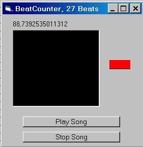
The “Beatcounter” helps with determining the beats per minute (bpm) of a song. On clicking this menu item, a dialog opens (Fig.70). This tool is also available in the Timeline Window via the menu “Tools”.
If a music file is loaded to the Timeline editor (via “New Show”), a click on “Play Song” starts playing it. Any key except Space or a right mouse click in the black area resets the counter. By either rhythmically left clicking in the black area or rhythmically pressing the space bar, the clicks are counted. Above the window the actually calculated bpm-rate is shown.
The red bar on the right side shows the tapping speed related to a calculated average, so if the red bar is above the black line, the tapping is too fast, if it’s below it’s too slow.
Click “Stop Song” to stop the sound output.
The longer the beat is recorded, the more precise is the calculated BPM.
6.18.8. Tool: Wave-Generator
The “Wave-Generator” is a special tool for automatically creating waves and other periodic figures. The tool appears to be complex, but it isn’t: It provides a multitude of features that result in stunning, automatically created animations that would take plenty of time if they would be created manually.
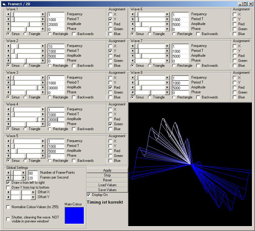
Fig.71: Extra Tools: Wave-Generator
The working principle of the Wave Generator is as follows (very technical, not directly necessary for just using the tool):
The Wave Generator consists of 8 single generators. Each can generate its own waveform. The amplitudes of the waveforms are dependent on space and time.
The amplitudes theoretically begin with a range from -100% to 100%, because the “real” amplitude (height of signal) at least arises from the combination with a point property (compare to “Wrench Tool” chapter 6.3.6). The amplitudes can be assigned to a point property like X/Y coordinates or color. All generators work in a similar way.
Every wave is characterized by amplitude, frequency (in space), period (in time) and phase.
The frequency describes the number of peaks and wave trough in the space. In Fig. 71 the frequency is 1 for wave 1 and it is assigned to the y coordinates with amplitude 20000. Thus the generated wave has 1 peak and 1 wave trough in total. The generator for wave 2 is also assigned to the y coordinates, but has a frequency of 10 and smaller amplitude of 5000. That generates the smaller wave with 10 peaks, which is interfering the big wave (see preview window in Fig.72).
The period T describes the time one point on the wave needs to reach the peak after being in the wave trough. The duration is entered in milliseconds. In the example in Fig.72 for the wave 1 the duration for one oscillation is 1000ms, thus it needs 1 second for the oscillating points to fulfil one complete period (to go up and come down again).
The amplitude describes the “intensity” of the wave (or the color when used). In other words: It describes the height and the depth of the peak and wave trough. The generator internally calculates in relative values (in %), because the amplitudes can be assigned to different point properties. Colors are described internally by values from 0 to 255 for each of the base colors RGB, coordinates can have values from -32767 to +32767. You see in Fig. 71 the big wave with amplitude 20000 and the interfering smaller wave with amplitude 5000. Furthermore you see in the picture the generators 3 and 4, which are assigned to red and green, respectively. Because they have the frequency 1 and amplitudes of 30000, they generate the white color (in combination with blue), which is partly dying the wave.
The phase describes, how much degrees the oscillation is shifted (in comparison to a wave with phase = 0). An example should explain the property of the phase: Let us take a sinus oscillation for the x-axis and for the y-axis, too. The result will be a line, rotated by 45° to the axes. To get a circle, we need a cosines oscillation for one of the axes. Now remember the basics of trigonometry: A cosine-function is the same as a sinus-function with a phase shift of 90° (when sin(x) = 1 then cos(x) = 0 and sin(x+90°) = 0 and the other way round).
All waves can be created as triangle- or rectangle-oscillations and the display can be altered in the direction (backwards), too.
HINT: The generator is designed to be very flexible. There were some requests of users to accept only certain conditions in order to simplify the handling. But this would restrict the flexibility. Because the flexibility has higher priority, some circumstances have to be taken into account:
Problem 1: Long times for calculations and very big files:
If values for the frequency and/or duration are used for the different generators, which are not integer multiples from each other, then the time to calculate the wave can be very, very long! Furthermore the size of the file significantly increases due to the large number of frames that need to be created.
Please feel encouraged to try and find out the effects of the very settings. It’s not necessary to calculate any frame numbers – just pay attention to the warning:

It is suggested to not exceed 1000 frames.
Global Settings:
The “Global Settings” apply to all generator tracks.
“Number of Frame Points” determines the number of points of the wave (of one frame).
“Frames per Second” adjusts the frame rate for the. This value can be changed later as well by adjusting the “Frames per Second”, see chapter 6.4.6. If the warning “Framecount >1000” is shown, reducing the frame rate to e.g. 30 may solve the problem of creating too many frames.
Activating “Draw x from left to right” creates a horizontally oriented wave (used in the example shown in Fig. 71).
Activating “Draw y from top to bottom” creates a vertically oriented wave.
Both options activated results in a diagonally oriented wave. If one of the options is chosen, then all amplitudes assigned to the other axis are ignored.
“Normalize Color Values (to 255)” sets the color values to at least have one of the laser sources in the laser operate at full power – this increases the visibility of the colors, but may change the color shade a bit.
The “Shutter” cleaves the waves to beams. The wave consists of many single beams following the course of the wave without having any links in between the points.
The button “Apply” starts the calculation of the wave and imports it to the Figure Table as figure 0. There it can be modified further (e.g. by applying morphing to get a smoother output) and saved to the hard disk.
The button “Preview” (toggles to “Stop” if Preview is active) displays a simulation of the created wave in the preview area. Another click on the button stops the simulation.
The button “Reset” resets all values.
The button “Load Values” allows for loading previously saved generator settings.
The button “Save Values” allows for saving wave generator settings.
6.18.9. Tool: Path Tool
A new animated multi-frame figure can be created with this tool, showing a moving frame alongside an animation path.
The tool consists of several modules for the input:
A) Input of Path
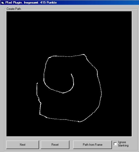
Fig. 72 shows the dialog for drawing the animation path. It is either possible to draw the animation path with the mouse or to import the animation path from the active figure in the figure editor by clicking “Path from Frame”. For verifying the results, activating of “Ignore Blanking” can help.
Hint:
The colors of the figure for the path (Path from Frame) can be transferred as well. Figures with color gradient can give very nice results.
To draw the path, click the button “Next” to go on with the process. If the drawing failed, click “Reset” to clear the window and try again. If the path shall be taken from a figure of the Figure Editor, it is useful to apply the function “Optimize Distance” via the menu Windows -> Special Features -> Opt.Distance to add intermediate points on straight parts of the path.
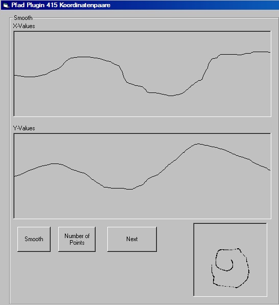
B) Path Edit Window
With the Path Edit Window (Fig. 73) it is possible to smoothen the course of the drawn path via the button “Smooth”. The number of points defining the path can be specified (button “Number of Points”). If the path was taken from a figure of the Figure Editor, it is usually not recommended to use the smoothening option, as the corners of the shape become round. After all editing has been done, click on the button “Next” to move on to the last module of the Path Tool.
C) Selection of Figure and Options
With this module (Fig. 74) the figure that shall move along the path can be selected. This can be the actively selected figure from the Figure Editor (Option “Source/ Use frame from main-window”) or a “Snake” line (Option “Source/Snake/Line”).
If “Snake” line is selected, a path line is created. The length of the path line is specified by the number entered in “Count of Pictures”.
If “Use frame from main window” is selected, the active figure from the Figure Editor will be displayed in the window of the module and thus is selected as figure for the movement on the path.
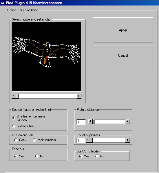
If the figure has not been chosen yet, it must be done at this point. If the window does not update the figure automatically, click on “Snake” and then again on “Use frame from main window”.
The red-green colored circle indicated the anchor point and can be positioned with a mouse click on the new position. This anchor point moves on the movement path later.
The “Use color from” option is used when creating a Snake line. It specifies if the color values are taken from the colored path (“Path”) or from the Figure Editor (“Main Window”).
Activating the option “Fade out” reduces the brightness (fades out) at the end of the path line or the last figures.
“Picture Distance” (upper scrollbar) specifies the distance of the points drawn for the path line, or, if a figure is moved, the distance between the copies of the figure.
“Count of pictures” (lower scrollbar) specifies the length of the path line or, if a figure is moved, the number of figure repetitions that are moved on the path.
“Start/End hidden” (blanking on start and end) specifies if the first and the last figure of the path are shown.
6.18.10. Tool: Stretch Lines Tool
The Stretch Line Tool creates a new, animated figure with multiple frames. This new animation must base on an existing figure (has to be active in the Figure Editor). The effects applied with the Stretch Lines Tool make the figure appear as just being drawn (lines are slowly appearing from the single points and end up as final figure)
“Line Stretch for each line” means that the drawing of the figure is simultaneously done from each point. Lines are drawn at the same time. Click “Apply” to use the effect with the active figure. The textbox allows for specifying the number of frames to be drawn.
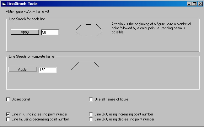
“Line Stretch for complete frame” starts drawing the figure in one point and then draws the lines until the figure is completed. Click “Apply” to use the effect with the active figure. The textbox allows for specifying the number of frames to be drawn.
If the option “Bidirectional” is checked, the figure is drawn line by line, and when it’s complete it is erased line by line again. (reverse order of the drawing).
The option “use all frames of figure” is applicable for multiframe figures only. If this option is checked, the next frame of the source figure is used for the next drawing step.
The options “Line in, using increasing (decreasing) point number” are used to specify the creation type of the figure. “Increasing” or “decreasing” defines the direction of the process.
The options “Line out, using increasing (decreasing) point number” are used to let the figure slowly disappear. “Increasing” or “decreasing” determines the direction of the process.
6.18.11. Tool: Bitmap Trace Tool
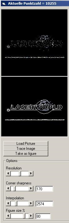
The Bitmap Trace Tool allows for easy conversion of simple logos and graphics to ILDA readable files. The more complex the picture, the more difficult is it for the software to output a proper result. Best results can be achieved with using line graphics.
Adaptions to the way Showeditor interprets and converts the pictures can be made by adjusting the slider settings in the tool window.
This is how it works:
First load a picture by using the button “Load Picture”. Then click on “Trace Image” to start the tracing. With the tracing the system tries to automatically convert the pixel image to a vector graphics.
To avoid getting a flickering projection later, it is recommended to not exceed a limit of 2000 points in total for a 30kpps Galvo system.
The number of “trace points” can be controlled with the four scrollbars: Moving them to the right means “more points”, to the left means “fewer points”.
The challenge is to find the ideal setting with as few points a possible but still achieving a good result.
It is helpful if the image that shall be converted has a width of about 800px and any unnecessary parts should have been already deleted with graphics software prior to tracing.
If the converted result is acceptable and shall be imported, a click on “Apply to figure” creates the respective figure in the drawing area of the Figure Editor.
6.18.12. Tool: Color Shove
The Color Shove tool creates a multi-frame animated figure from a single frame by animating the colors of the figure: The different colors are shoved through the figure point by point (one point per frame), so the figure gets kind of a color sparkling effect – but only with the colors it consists of.
Example of how this tool works:
A triangle is given – side 1 is red, side 2 is green and side 3 is blue. In total there are 3 colors (4, if the blanked points are respected). When applying the Color Shove, a new figure is created consisting of 3 (4) frames. The triangle shape remains the same, but on each change of a frame, the respective color moves on by one point. So the sides of the triangle change their color by every frame change.
This of course also works with more complex graphics. As the tool only uses the colors already present in the figure, the animation created by the Color Shove looks homogenous and matches the general color set.
The Color Shove Tool also works for multi frame figures, but only the colors of the first frame are shifted. For the following frames the original x/y coordinates of the animation stay the same, but the colors set from the first frame is pushed through. Due to this it is necessary that the number of points should be the same per frame, otherwise the software needs to interpolate points that are missing – which may lead to unwanted results.
Hint:
To decrease the distance between points, it is recommended to use the “Opt. Distance” tool. (See chapter 6.3.6, shown in Fig.77).
Important:
For using the tool, an already existing and saved figure is needed. Remember to save all changes to an existing figure prior to applying this tool!
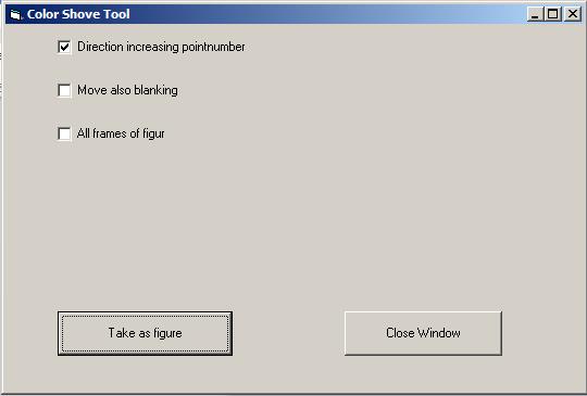
Fig.77: Extra Tools: Color Shove
When using the Color Shove Tool, several choices are possible:
● “Direction increasing point number”
This option determines the direction to shoving the colors.
● “Move also blanking”
When active, also the blanked points are shoved (the property “invisible” is regarded as color and is shoved through the figure).
● “All frames of figure”
This option works for multi-frame figures. It adds a special color shove, consisting of two effects:
1) The colors of the first frame are shifted through all points the frames created by the Color Shove Tool.
2) The coordinates of the points reference to the ones in the existing frames of the figure.
It is recommended to test the different features of the Color Shove Tool to understand their behaviour and to learn more about their potential.
6.18.13. Tool: Insert Color Gradient / Insert Smooth Colors
This tool inserts a color gradient to the figure. There is already an option “Use Soft Color” within the Effects Window (See chapter 4.3.) and indeed, this function does the same, except for one main difference: The “Use Soft Color” effect is processed just before the output of the figure. If it is e.g. intended to shift colors of a figure with color gradient or to use a colour gradient for the path tool, then “Use Soft Colour” has no effect.
The Insert Color Gradient Tool allows for directly creating color gradients and adding them to the figure. As the color gradient is then applied to the very frame, further tools and modifications can be applied with respect of the applied gradient.
It is necessary that the active figure has been saved, before applying the tool.
With using the tool a new figure is created. A dialog opens, asking for the desired transition effect for the color gradient.
Fig.78: Extra Tools: Dialog of “Insert Color Gradient”
6.18.14. Live Window
Opens the Live Window (See chapter 12).